Neural Networks

Introduction

Neural networks are powerful machine learning models capable of performing both classification and regression tasks (by changing the loss function). They represent a convergence of several key concepts in machine learning, including:

• Perceptrons: The foundational single-layer neuron model.
• Logistic Regression: Often used for activation functions and output layers in classification.
• Ensemble Learning: Conceptually similar in how layers build upon each other.
• Stochastic Gradient Descent (SGD): The primary method used for training NNs.
• Feature Engineering: NNs automate the process of discovering relevant features from raw data, unlike methods where features must be explicitly defined.

Historically, early research on perceptrons (like Rosenblatt’s work in 1957) faced setbacks (the first “AI Winter”) partly due to limitations highlighted by Minsky and Papert, such as the inability of a single perceptron to solve the XOR problem. Modern NNs overcome these limitations through layered architectures and non-linear transformations.

Intuition: Overcoming Linearity

The Perceptron Limitation: The XOR Problem

A single perceptron computes a linear combination of its inputs and applies a threshold. This means it can only separate data that is linearly separable. The classic example of a non-linearly separable problem is the XOR function:

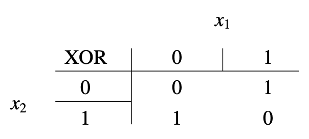
It’s impossible to draw a single straight line (in 2D) to separate the points labeled ‘1’ from those labeled ‘0’.

Solutions to Non-Linearity:

1. Manual Feature Engineering: One way to solve XOR is to add a new, non-linear feature, like $x_1\ast x_2$. In the resulting 3D space ($x_1,x_2,x_1\ast x_2$), the XOR points become linearly separable. However, finding the right features manually is difficult for complex problems.
   
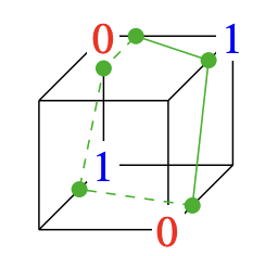
   This is a drawing of what the XOR function would look like in 3D, with the new $x_1\ast x_2$ feature being the third dimension (represented as the direction coming towards you). The top left corner of the cube, farthest away from you, is $(0,0,0)$. The bottom right corner, closest to you, is $(1,1,1)$.

2. Layered Architecture + Non-Linearity: Neural networks solve this by:

   • Layering: Using the outputs of one set of linear classifiers (neurons) as inputs to another layer.
   • Non-Linearity: Crucially, applying a non-linear activation function after each layer’s linear combination. Without non-linearity, stacking linear layers just results in another linear function ($a(bx+c)+d$ is still linear in $x$).

With non-linearity, neurons can act like logic gates, allowing networks to approximate complex, non-linear functions, including XOR.

More Intuition: Stitching together ReLUs

Neural networks with ReLU activations can approximate complex functions by stitching together simple linear pieces.

• For example, we can approximate a smooth sine wave using piecewise linear predictions.

To build a piecewise linear function, we can use the ReLU activation function:

$$f(x)=max(0,x)$$

We think of this as an “elbow”:

• Left of the elbow: flat (zero)
• Right of the elbow: linear (slope = w)

We control the shape of the ReLu unit with:

1. Slope (w) — controls the steepness after the elbow
2. Elbow position — determined by the bias term b
3. Whether we “turn on” the elbow or not — through the input range

Given:

$$f_{w,b}(x)=max(0,w\cdot x+b)$$

• Elbow position (x where the output becomes non-zero): $$x=-\frac{b}{w}$$ ​
• Slope to the right of the elbow: $$slope=w$$

So by adjusting w and b, we shift and shape the elbow to approximate different parts of a target function.

To move the elbow, change:

• The weight (w) — affects the angle
• The bias (b) — shifts it horizontally

This is implemented as:
Input x → [multiply by w] → [add b] → ReLU → output

$$f(x)=max(0,w\cdot x+b)$$

This ReLU block is a small piece of a bigger function approximator.

The full neural network consists of:

• Input Layer: raw input features
• Hidden Layer: uses ReLU activations to add non-linearity
• Output Layer: often linear, especially for regression problems

Each neuron computes:

$$f(x)=max(0,w\cdot x+b)$$

The hidden layer assembles many of these elbows to approximate the target function.

The optimizer (like SGD or Adam) minimizes a loss function (e.g., MSE):

$$L=(y_{pred}-y_{target}{)}^2$$

During training:

• The optimizer updates weights and biases
• This shifts the location and slope of the elbows
• The process continues backward, using gradients to find how to best move $w,b$ to lower the loss

This is how neural nets learn to “carve out” a function that closely fits your data.

---

Neural Network Architecture

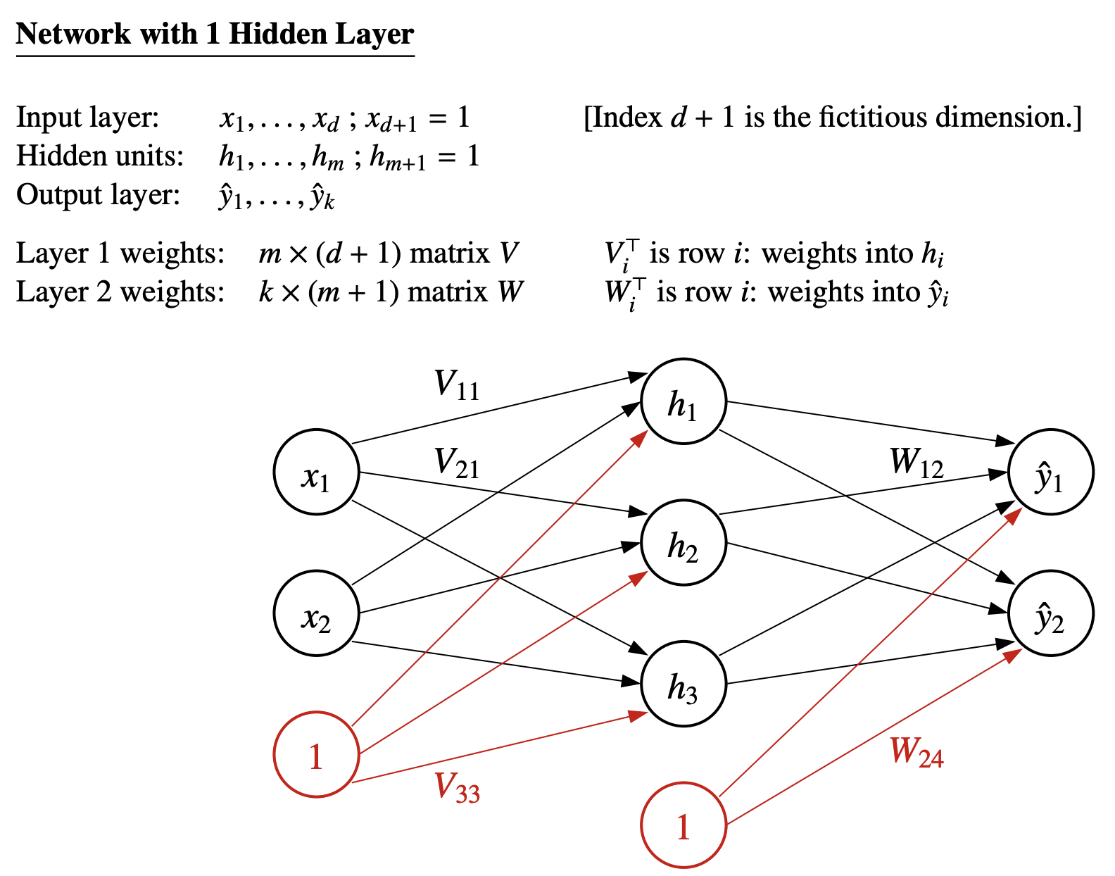
A typical feed-forward neural network consists of:

1. Input Layer: Receives the raw data features (e.g., $x_1,...,x_d$). Often includes a bias unit (conceptually $x_{d+1}=1$) which allows the neuron to learn an offset.
2. Hidden Layer(s): One or more layers of neurons between the input and output. These layers learn intermediate representations of the data. Each hidden layer also typically includes a bias unit ($h_{m+1}=1$). The number of hidden layers defines the network’s “depth”. Common image recognition networks might have 8 to 200+ hidden layers.
3. Output Layer: Produces the final prediction(s) (e.g., class probabilities $z1,...,zk$ or a regression value).

Neurons, Weights, and Activation Functions

• Neurons (Units): Each node in the hidden and output layers. It computes a weighted sum of its inputs and then applies an activation function.
• Weights: Parameters associated with the connections between neurons in adjacent layers. These are what the network learns during training.
  • $V$: Weight matrix connecting the input layer to the first hidden layer. $V_i$ is the vector of weights into hidden unit $h_i$.
  • $W$: Weight matrix connecting the last hidden layer to the output layer. $W_j$ is the vector of weights into output unit $z_j$.
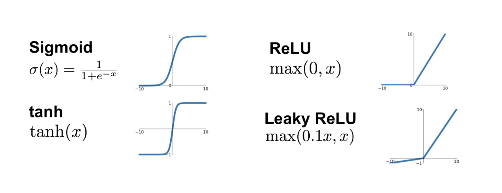
• Activation Functions: Non-linear functions applied element-wise to the weighted sum at each neuron. Common choices include:
  • Sigmoid (Logistic): $s(\gamma )=\frac{1}{1+e^{-\gamma }}$. Squashes output between 0 and 1. Historically popular, but prone to “vanishing gradients”.
  • ReLU (Rectified Linear Unit): $r(\gamma )=max(0,\gamma )$. Computationally efficient and often performs better in deep networks, though can suffer from “dying ReLUs” and potentially “exploding gradients”.
  • Softmax: Used for multi-class classification output layers to produce probability distributions. $softmax(z_i)=\frac{e^{z_i}}{{\sum }_{j=1}^K{e}^{z_j}}fori=1,2,\dots ,K$ where $z$ is the pre-activation values for the output layer.
    

The Forward Pass

This is the process of making a prediction for a given input $x$:

1. Input to Hidden: Calculate the pre-activation values for the hidden layer by multiplying the input vector $x$ (including the bias term) by the first weight matrix $V$.
   • $a_h=V\ast x$
2. Hidden Activation: Apply the hidden layer’s activation function (e.g., ReLU or Sigmoid) element-wise to the pre-activation values $a_h$. Append a bias term (1) to the resulting hidden activation vector $h^{\prime }$.
   • $h^{\prime }=hiddenActivation(a_h)$ (element-wise)
   • $h_{biased}=[h^{\prime },1]$
3. Hidden to Output: Calculate the pre-activation values for the output layer by multiplying the activated (and biased) hidden layer vector $h_{b}iased$ by the second weight matrix $W$.
   • $a_z=W\ast h_{biased}$
4. Output Activation: Apply the output layer’s activation function (e.g., Sigmoid, Softmax, Linear) element-wise to the pre-activation values $a_z$ to get the final prediction $z$.
   • $z=outputActivation(a_z)$ (element-wise)

For example:

For a network with one hidden layer using sigmoid activation ($s(z)=\frac{1}{1+e^{-z}}$) everywhere:

• $h=s_1(Vx)$ ($s_1$ applies sigmoid via component-wise calculation aka $h_i=s(V_1\cdot x)$ and appends a 1 for bias)
• $\hat{y}=s(Wh)=s(W{s}_1(Vx))$

A single fully-connected neuron: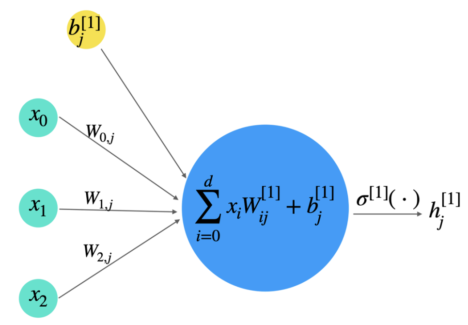

---

Training Neural Networks

The goal of training is to find the optimal weight matrices (V, W, etc.) that minimize the difference between the network’s predictions ($z$) and the true labels ($y$) across the training dataset.

Key Components

1. Loss Function $L(\hat{y},y)$: Measures the error for a single data point. Examples:
   • Squared Error: $L(\hat{y},y)=||\hat{y}-y|{|}^2$. Common for regression with linear output units.
   • Logistic Loss (Binary Cross-Entropy): $L(\hat{y},y)=-[y\ast ln(\hat{y})+(1-y)\ast ln(1-\hat{y})]$. For binary classification with a sigmoid output.
   • cross-entropy loss: $L(\hat{y},y)=-{\sum }_{i=1}^M{y}_i\ln ({\hat{y}}_i)$. For multi-class classification with a softmax output (assumes y is one-hot encoded or sums to 1). Strongly recommended over squared error for classification outputs as it helps mitigate vanishing gradients in the output layer.
2. Cost Function $J(V,W)$: The average loss over the entire training dataset (or a batch). $J=\frac{1}{n}{\sum }_{i=1}^{n}L(\hat{y}(X_i),Y_i)$.
3. Optimization Algorithm: Typically Gradient Descent (or variants like SGD, Adam, etc.). The weights are iteratively updated in the opposite direction of the gradient of the cost function.
   • $w_{new}=w_{old}-\epsilon \ast \nabla J(w)$ (where $w$ represents all weights $V,W$).
   • $\epsilon$ is the learning rate.
   • Batch GD: Uses the gradient calculated over the entire dataset.
   • Stochastic GD (SGD): Uses the gradient calculated from a single randomly chosen data point at each step. Faster updates, noisier gradient, can help escape local minima. Often used with mini-batches.

Challenges in Training

• Non-Convexity: The cost function $J$ is typically highly non-convex, meaning it has many local minima. Gradient descent might converge to a suboptimal local minimum. Having sufficiently large hidden layers often helps find good solutions in practice.
• Symmetry: If all weights are initialized to the same value (e.g., zero), all neurons in a layer will compute the same thing, and the gradients will be identical. The network cannot learn effectively.
• Initialization: Weights must be initialized randomly to break symmetry. They should also be small (e.g., drawn from a distribution with mean 0 and standard deviation $1/sqrt({fan}_{in})$) to prevent initial saturation of sigmoid units or overly large activations with ReLUs.
• Vanishing Gradients: In deep networks with sigmoid/tanh activations, gradients can become extremely small as they propagate backward, making learning in earlier layers very slow or stagnant (“stuck” units).
• Exploding Gradients: Gradients can become excessively large, especially in deep or recurrent networks (often with ReLUs), leading to unstable training (large weight updates). Gradient clipping is a common mitigation technique.

---

Backpropagation

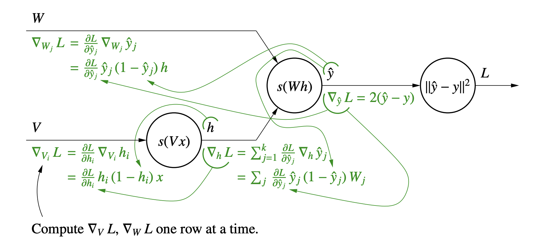
Backpropagation is the algorithm used to efficiently compute the gradient of the cost function ($\nabla J$) with respect to all weights (V, W) in the network. It avoids redundant calculations by using the chain rule and dynamic programming.

1. Forward Pass: Compute the activations for all layers, starting from the input $x$ and progressing to the final output prediction $\hat{y}$. Store the intermediate values.
2. Backward Pass: Compute the gradients starting from the output layer and propagating backward towards the input layer.
   • Calculate the gradient of the Loss with respect to the output activations (${\nabla }_{\hat{y}}L$).
   • Use the chain rule to find the gradient of the Loss with respect to the output pre-activations (${\nabla }_{h}L$).
   • Use this to find the gradient of the Loss with respect to the weights connecting to the output layer (${\nabla }_{W}L$).
   • Use ${\nabla }_{\hat{y}}L$ and ${\nabla }_{h}L$ along with intermediate gradients (like ${\nabla }_{W_j}{\hat{y}}_j$ and ${\nabla }_{V_i}{h}_i$) to compute the gradients with respect to the weights, ${\nabla }_{W}L$ and ${\nabla }_{V}L$.
   • Repeat this process, propagating the gradients backward layer by layer until the gradients with respect to all weights are computed.

Efficiency

Backpropagation computes the entire cost gradient $\nabla J$ in $O(E)$ time, linear in the number of weights (edges) $E$. This is significantly faster than the naive $O(E^2)$ approach of calculating each weight’s gradient independently.

Note: All figures in this note are taken from UC Berkeley’s CS 189 class lecture notes.

References

CS 189, Lecture 16
CS 189, Lecture 17
CS 189, Lecture 18
CS 189, HW 6